Here we derive a simple characterization of predicting a vector of unknown stochastic variables using observed data that is essentially regression using population statistics rather than using a sample proxy. Anderson (2004), Hamilton (1994) and many multivariate statistics textbooks contain similar treatments.
4.1.1 Unconditional moments
Let \(z\) be vector of stochastic variables such that \[
z\sim N(\mu,\Sigma)
\] or \[
\mathbb{E}\left[ \left(z-\mathbb{E}[z]\right) \left(z-\mathbb{E}[z]\right)' \right] = \mathbb{E}\left[ \left(z-\mu\right) \left(z-\mu\right)'\right] = \Sigma
\] Divide the vector into two, \(z_1\) and \(z_2\) so that \[
\begin{bmatrix}
z_1 \\
z_2
\end{bmatrix}
\sim N\left(
\begin{bmatrix}
\mu_1 \\
\mu_2
\end{bmatrix},
\begin{bmatrix}
\Sigma_{11} & \Sigma_{12} \\
\Sigma_{21} & \Sigma_{22}
\end{bmatrix}
\right)
\] The unconditional covariance of \(z_1\) is unaffected by the known covariance between it and \(z_2\), \(\Sigma_{12}\).
4.1.2 Conditional mean for \(z_1\)
How do we best use the information in an observed part of the vector \(z\) – say \(z_2\) – to better predict the unobserved part?
Assume there is linear relationship between the two \(z\) variables such that \[
z_1 = Bz_2 + \varepsilon\qquad \text{or}\qquad \varepsilon =z_1-Bz_2
\] Now choose \(B\) such that \(\varepsilon\) and \(z_2\) are uncorrelated – a value of \(B\) where this holds is a fundamental assumption for a regression model as it implies there is no useful information in \(z_2\) that we aren’t using. This implies \[
\begin{aligned}
0 &= \mathbb{E}\left[ \left(\varepsilon - \mathbb{E}[\varepsilon ]\right) \left(z_2 - \mathbb{E}[z_2]\right)'\right]\\
&= E\left[ \left(z_1 - Bz_2 - \mathbb{E}[z_1-Bz_2]\right) \left(z_2 - \mathbb{E}[z_2]\right)'\right] \\
&= E\left[ \left(z_1 - \mu_1 - B\left(z_2-\mu_2\right) \right) \left( z_2-\mu_2\right)'\right] \\
& =\Sigma_{12}-B\Sigma_{22}
\end{aligned}
\] We recover \(B=\Sigma_{12}\Sigma_{22}^{-1}\). This is simply regression using a ‘method of moments’ characterization where we use population rather sample moments. For known conditioning values \(z_2\) and known \(\Sigma_{12}\), \(\Sigma_{22}\)\[
\begin{aligned}
\mathbb{E}\left[ z_1|z_2\right] &= \mathbb{E}\left[ Bz_2+\varepsilon |z_2\right] \\
&= Bz_2 + \mathbb{E}\left[\varepsilon \right] \\
&= Bz_2 + \mathbb{E}\left[z_1-Bz_2\right] \\
&= B z_2 + \mu_1 - B \mu_2 \\
&= \mu_1 + B(z_2-\mu_2)
\end{aligned}
\] Plugging in the formula for \(B\) gives the conditional expectation of \(z_1\) given \(z_2\) as \[
\mathbb{E}[z_1 | z_2] = \mu_1 + \Sigma_{12} \Sigma_{22}^{-1}(z_2-\mu_2)
\] This is a formula that updates the unconditional expectation by a weighted average of the “innovation” (deviation from predicted value) of the observed variables.
4.2 Example
As an example, consider the \(4\times 4\) covariance matrix \(\Sigma\)
\[
\Sigma = \left[\begin{array}{r}1.28 &1.74 &-0.25 &-0.52 \\1.74 &10.16 &-4.79 &3.12 \\-0.25 &-4.79 &4.44 &-1.86 \\-0.52 &3.12 &-1.86 &2.42 \\\end{array}\right]
\] It is a simple matter to generate four sample sequences with this covariance. We set the constants \(\mu_i^j = 0\) for \(i,j = 1,2\) as we subtract them out anyway.
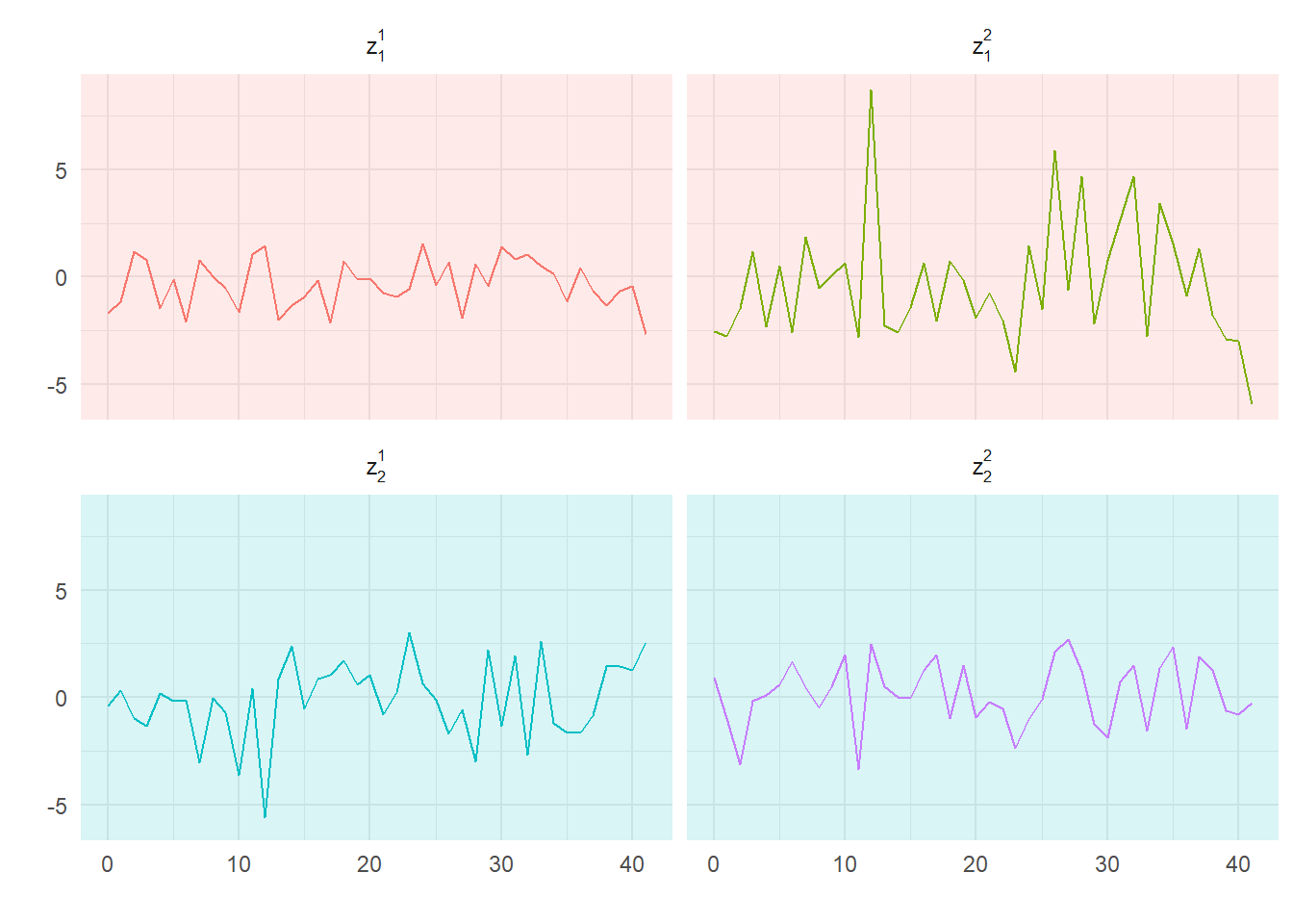
Four sample series with covariance matrix \(\Sigma\)
Denote the first two series \(z_1^1\) and \(z_1^2\), and the second two \(z_2^1\) and \(z_2^2\); thus \(z_1\) from earlier is a vector of the first two (\(z_2^1\) and \(z_2^2\)) and \(z_2\) a vector of the second two (\(z_2^1\) and \(z_2^2\)).
4.2.0.1 Problem
If we know \(\Sigma\), and can observe these last two series (on light blue backgrounds), how well can we reconstruct the first (light red backgrounds) two ?
4.2.1 Solution
Calculate \(B\) from the above formula. By inspection \[
\Sigma_{22} = \left[\begin{array}{r}4.44 &-1.86 \\-1.86 &2.42 \\\end{array}\right]
\] and \[
\Sigma_{12} = \left[\begin{array}{r}-0.25 &-0.52 \\-4.79 &3.12 \\\end{array}\right]
\] so \(B = \Sigma_{12}\Sigma_{22}^{-1}\) is \[
B = \left[\begin{array}{r}-0.214 &-0.377 \\-0.795 &0.679 \\\end{array}\right]
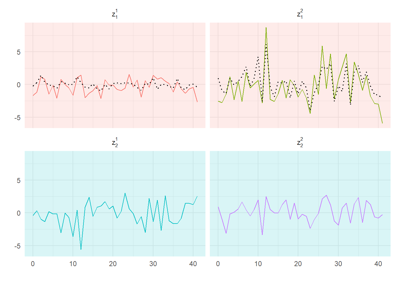
\] Calculating the predicted variables and plotting them on the same graph we get
ZZfit <-data.frame(Z[,3:4] %*%t(B), x =0:(nobs-1)) %>%rename_all(~c("z11", "z12", "x")) %>%gather(Var, Fit, -x) %>%mutate(F =as_factor(Var), F =recode_factor(F, z11="z[1]^1", z12="z[1]^2"))ZZhat <-left_join(ZZ, ZZfit)
Plots of actual and predicted first and second series
where the correlations between the variables and their fitted values are 0.59, 0.76 respectively.
4.2.2 Observing different \(z\) variables
What if instead of observing both of the last \(z\) variables we only observe one, say the last one? Nothing we have said so far restricts us from having only one observable, or three – and of course ordering is arbitrary.
Lets assume we just see the last variable. Calculate \(B\) from the above formula. As before, by inspection \[
\Sigma_{22} = \left[\begin{array}{r}2.42 \\\end{array}\right]
\] and \[
\Sigma_{12} = \left[\begin{array}{r}-0.52 &3.12 &-1.86 \\\end{array}\right]'
\] and as now \(\Sigma_{22}\) is a scalar we can write \(B = \Sigma_{12}/\Sigma_{22}\) which is
B <- Sigma[1:3,4, drop=FALSE]/Sigma[4,4]
\[
B = \left[\begin{array}{r}-0.213 &1.289 &-0.766 \\\end{array}\right]'
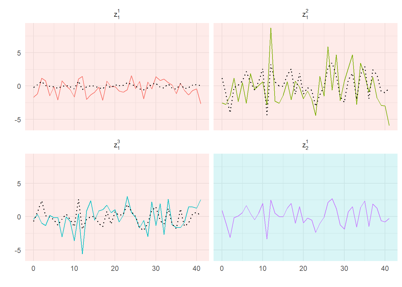
\] Applying this we get predictions of the three unknown variables which are
Plots of actual and predicted series, one predictor
where we have color coded the backgrounds accordingly. In general, predictions are usually a bit worse, but sometimes almost as good – and may even look a bit better! Comparing them to our previous results the correlations between the variables and their predicted values are now 0.34, 0.51, 0.43 respectively, where of course we are predicting one more series now.
4.2.3 Remarks
Depending on the covariance matrix, correlation can be a lot lower. If the \(z_1\) and \(z_2\) vectors are uncorrelated then \(\Sigma_{12}\approx 0\) so \(B\approx 0\).In these circumstances the best prediction is then close to the unconditional mean; if \(\Sigma_{11}>0\) then predictions will be poor although the absolute value of those errors depends on \(\Sigma_{11}\).
This also illustrates that there are some variables that are better at predicting the things you are interested in than others. It practice it is frequently the case that there is low correlation between predicted and actual – as ever, you need good regressors to get a good fit between predicted and actual.
4.3 Updating the update and assessing uncertainty
4.3.1 Updating an estimate with new information
This result easily generalizes: what if we already have an estimate but we get some new information that we could use to improve our estimate? We can solve this using the formula we have already derived. In effect we can divide \(z_2\) and include some further variables denoted \(v\) such that \[
\begin{bmatrix}
z_1 \\
z_2 \\
v
\end{bmatrix}
\sim N\left(
\begin{bmatrix}
\mu_1 \\
\mu_2 \\
0
\end{bmatrix},
\begin{bmatrix}
\Sigma_{11} &\Sigma_{12} & \Sigma_{1v} \\
\Sigma_{21} &\Sigma_{22} & 0 \\
\Sigma_{v1} & 0 & \Sigma_{vv}
\end{bmatrix}
\right)
\] Notice we have imposed that \(v\) is mean zero (\(\mu_v = 0\)) and uncorrelated with \(z_2\) (\(\Sigma_{v2} = \Sigma_{2v}'=0\)). It is important that they are uncorrelated with previous conditioning variables but not the variables to be predicted so \(\Sigma_{1v}\ne 0\). In this way \(v\) represents news. We couldn’t have predicted it from information we already had.
Conditioning \(z_1\) on \((z_2,v)\) we get \[
\begin{aligned}
\mathbb{E}[z_1|z_2,v] &= \mu_1 +
\begin{bmatrix} \Sigma_{12} & \Sigma_{1v} \end{bmatrix}
\begin{bmatrix} \Sigma_{22}^{-1} & 0 \\ 0 & \Sigma_{vv}^{-1} \end{bmatrix}
\begin{bmatrix} z_2-\mu_2 \\ v \end{bmatrix} \\
&= \mu_1 +\Sigma_{12}\Sigma_{22}^{-1}(z_2-\mu_2)+\Sigma_{1v}\Sigma_{vv}^{-1}v
\end{aligned}
\] We can further write this \[
\mathbb{E}[z_1|z_2, v] = \mathbb{E}[z_1|z_2] +\Sigma_{1v} \Sigma_{vv}^{-1}v
\]
4.3.2 Covariances
So far concentrated on the expected value, but can similarly construct the conditional covariance. The conditional variance for the \(z_1\) given \(z_2\) is \[
\begin{align}
var(z_1|z_2) &= \mathbb{E}\left[\left(z_1 - \mathbb{E}(z_1|z_2) \right) \left(z_1 - \mathbb{E}(z_1|z_2) \right)' \right] \\
&= \mathbb{E}\left[ \left(z_1 -\mu_1-\Sigma_{12}\Sigma_{22}^{-1}(z_2-\mu_2) \right) \left(z_1-\mu_1 -\Sigma_{12}\Sigma_{22}^{-1} (z_2-\mu_2) \right)' \right] \\
&= \Sigma_{11}-\Sigma_{12}\Sigma_{22}^{-1}\Sigma_{21} + \Sigma_{12}\Sigma_{22}^{-1}\Sigma_{22}\Sigma_{22}^{-1}\Sigma_{21} - \Sigma_{12}\Sigma_{22}^{-1}\Sigma_{21} \\
&= \Sigma_{11}-\Sigma_{12}\Sigma_{22}^{-1}\Sigma_{21}
\end{align}
\] so \[
var(z_1|z_2) = \Sigma_{11}-\Sigma_{12}\Sigma_{22}^{-1}\Sigma_{21}
\] This tells us that the conditional covariance can be no bigger than the unconditional one. We get an efficiency gain.
When we consider updating the covariance of a conditional expectation it follows that \[
\begin{align}
var(z_1|z_2,v) &= \Sigma_{11}-
\begin{bmatrix} \Sigma_{12} & \Sigma_{1v} \end{bmatrix}
\begin{bmatrix} \Sigma_{22}^{-1} & 0 \\ 0 & \Sigma_{vv}^{-1} \end{bmatrix}
\begin{bmatrix} \Sigma_{21} \\ \Sigma_{v1} \end{bmatrix} \\
&= \Sigma_{11} - \Sigma_{12}\Sigma_{22}^{-1}\Sigma_{21} - \Sigma_{1v}\Sigma_{vv}^{-1}\Sigma_{v1} \\
&= var(z_1|z_2) - \Sigma_{1v}\Sigma_{vv}^{-1}\Sigma_{v1}
\end{align}
\] It follows that the covariance here must be no bigger than the variance conditioned on \(z_2\) alone, consistent with our previous result.
Anderson, T. W. 2004. An Introduction to Multivariate Statistical Analysis. 3rd ed. New York: John Wiley; Sons.
Hamilton, James D. 1994. Time Series Analysis. Princeton, NJ: Princeton University Press.